dt.pepperdine.edu

Evaluation of Neural Networks for Automatic Target Recognition

K. Wojtek Przytula

Hughes Research Laboratories, RL69

3011 Malibu Cyn. Rd

Malibu, CA 90265

ph. (310) 317 5892, fax (310) 317 5484,

e-mail: wojtek@msmail4.hac.com

Don Thompson

Pepperdine University

Department of Mathematics

Malibu, CA 90 263

ph. (310) 456 4831, fax (310) 456 4785,

e-mail: thompson@pepperdine.edu

ABSTRACT

In automatic target recognition we often face a problem of having to train a large neural network using a very limited data set. The paper presents methods designed to analyze trained networks. The methods allow to investigate how the network makes its decisions and what are its generalization properties. The methods interact with each other and are intended to be used as a complete set. They use techniques of sensitivity analysis, linear algebra, and rule extraction. They have been coded in Matlab as a toolbox and tested on a large number of real networks.

1. INTRODUCTION

One of the most important problems in aerospace, and at the same time one of the hardest to solve, is the problem of Automatic Target Recognition (ATR). The targets include air, land, and sea objects, which are classified using signals from a whole range of sensors such as radar (including SAR), infrared (e.g. FLIR), vision, sonar etc.. Recently neural network classifiers have been proposed for ATR with a significant degree of success. The issue hampering effective application of neural networks to most types of ATR is lack of large representative data bases, because of very high cost of data acquisition. Moreover, the data are often very complex and difficult to classify. The extraction of features from such data leads to large feature vectors. This in turn imposes large size of the input layer of the neural network. Consequently, we face a predicament of having to train a large network using a small set of examples. A very natural issue in this context is the reliability of the trained network. Lack of complete trust forces us to us look inside of the network, which throughout the training and testing appears to us as essentially a "black box".

Most of the efforts in the neural network research community have been concentrated on development of proper network design techniques. These techniques assist in selecting the right training algorithm, in defining appropriate topology of the network and help in providing best performance for both training and testing set. In our approach it is assumed that the design and training of the network have been already completed. What we are proposing is a set of techniques for evaluation of the trained network. The techniques are applicable to all multilayer networks without feedback. Throughout the paper we terminology most suitable for neural network classifiers, e.g. class boundary, class generalization etc. ; however the techniques of the paper are suitable to analyze networks for other applications as well.

Our goal is to find such characteristics of a trained network, which would provide a clear and compact interpretation of the network behavior. In particular we are interested in learning how individual inputs affect the output of the network (e.g. which are decisive in classifying inputs), how neural network separates input space into classes i.e. what is the shape of the class boundaries and the network behavior in their vicinity, how well the network generalizes beyond the exemplars it was trained on. In order to accomplish this goal we apply an integrated approach based on three types of methods: sensitivity analysis, algebraic methods, and rule extraction.

In sensitivity analysis we view the neural network as a multivariate vector function y = N ( W, x ), which maps input vector x Î X, X input space , into y Î Y, Y output space . The function is parametrized by the weight matrix W and is fully defined once the network is trained. In ATR applications, as in most other applications, a high dimensionality of the input space makes a simplistic tabulation approaches useless for characterizing the function. We have therefore developed a range of techniques, which when used together provide a good insight into the sensitivity of the function to individual inputs, behavior near the class boundaries in input space and generalization properties. Utility of the sensitivity techniques can be enhanced by a preparatory analysis of the input space. Such an analysis would combine a priori information about the input space resulting from the specifics of the problem (e.g. type of sensor, preprocessing used, application scenario) with computation of input data distributions, clusters, centroids, outliers, etc. Nevertheless the discussion of the input space analysis is beyond the scope of this paper.

There are several results known in literature , which are related to some of the sensitivity techniques discussed in this paper, [1], [2]. However, their fragmentary nature prevents them from being very effective for networks analysis. Our experiences with a large number of real networks has shown that a broader range of techniques combined with a coherent methodology is needed for analysis of networks.

The second class of methods - the linear algebraic methods - complements the results obtained by sensitivity analysis to improve understanding of the shape of classification boundaries and the generalization properties of the network. The linear methods limit our investigation to a single layer of a neural network, because the entire network is highly nonlinear. In particular we analyze the matrix of weights between input and hidden neurons and the covariance matrix of the hidden layer activations. Other authors looked at these matrices in the context of network training . In [3] and [4] a method was proposed for reconfiguration of a network to reduce the training requirements. In [5] a criterion is presented, which allows to determine when it is appropriate to stop the training.

Our third class of methods encompasses techniques for extraction of rules from trained networks. These are rules of the type: if input vector x belongs to a given region R then it is a member of a specific class i.e. the output of the network will indicate membership of that class. The rules approximate the actual class regions, and thus provide information about the class boundaries as acquired by the trained network. We are using multidimensional intervals as the rule regions R similarly to [6], however our rule generation algorithms are novel. Alternative approaches to the rule extraction are discussed in [7].

The various techniques constituting the three above classes of methods have been captured in form of algorithms in an integrated software toolbox. The toolbox has been coded in Matlab and tested on a large number of networks. It has shown to be very effective for analysis of trained networks providing the user a good understanding of the internal working of the "black box" representing the neural networks in training.

The paper consists of five chapters. After introduction in chapter 1 we present sensitivity analysis methods in chapter 2, algebraic methods in chapter 3, and rule extraction in chapter 4. The paper ends with conclusions in chapter 5.

2.0 SENSITIVITY ANALYSIS

2.1 Approach

Trained neural network can be viewed as a multivariate vector function

y = N ( W, x ) , (1)

where x Î X is and input vector from input space X, y Î Y is an output vector from output space Y, W is a matrix of parameters (weight matrix). In a typical ATR application, as in most other applications, the input space has between 5 to 50 dimensions. The output space is often also multi-dimensional. All the methods presented in the sequel apply to networks with multiple outputs, however for simplicity of presentation we will assume that there is only one output. We will also assume that the inputs and the output are normalized to a closed interval [0,1]. Value 1 on the output is reached for one class of inputs ( high-value class) and value 0 for the other class (the low-value class). The output value .5 is assumed to be the threshold value separating the two classes, and is therefore obtained for all the points in the input space, that represent the class boundaries . These are the boundaries acquired by the network in the process of training. They approximate the actual boundaries in the input space. The quality of this approximation depends on the choice of network topology, network training and how well the exemplars used in training represent the reality of the data.

We are interested in input-output relation of the function as it affects the classification. In particular we would like to know ,which inputs matter most in the classification decision, what is the function like near the class boundaries, and what could we say about expected generalization properties. The network function is fully defined once the training is completed, thus we can easily obtain the value of function output , and know its classification , for any input. Nevertheless simple tabulation of the function even in limited subregions of the input domain are hard to interpret, because of high dimensionality of the input space. The problem is therefore to extract easy-to-interpret information about the function , which provides insight into its important characteristics.

It is desirable to precede the analysis of the network function N with a good understanding of the structure of the input space. From the idiosyncrasies of the problem, e.g. type of sensor used, preprocessing of sensor input, data acquisition scenario, we can obtain some information about the input space. This information needs to be augmented by statistical analysis of the input data. We are interested in distributions of both, their clustering characteristic (centroids, outliers, etc.). We will not elaborate on data analysis techniques, however it is important to remember that this analysis helps significantly in our main goal, which is network analysis. During the learning the network acquires the structure of the data from the exemplars. By comparing what we see in the data and what the network learned, we can better judge the network.

2.2 Methods

In this section we describe the specific methods of extracting information about the network function N, which will characterize: the dependence of network classification decisions on the individual inputs, the behavior of the function near the class boundaries, and the generalization properties of the network. The network function is a very complex and highly nonlinear function defined over a region of high dimensionality. Any single method provides only a very limited insight into the function. It takes a combination of the methods presented in this section with the algebraic and rule extraction methods described in the two following chapters to get satisfactory picture.

The network function is obtained as a result of training, which is forcing it to be equal to 1 for one class of exemplars and to 0 for the other class. Thus the function takes on one of the two values 1 or 0 over most of its domain. The rest of the domain is providing space for output transition from 1 to 0, in it lie the boundaries separating the two classes. The behavior of the function in the vicinity of exemplars and in the boundary region tells us a lot about the generalization properties of the network.

Method 1

In this method we characterize the function along selected straight lines in its domain . This is a 1-D characterization of the multidimensional function. However, by selecting important points and running multiple straight lines through the points , e.g. running through the exemplars lines parallel to all the coordinate axis, we obtain information about behavior of the function in some vicinity of the points. The 1-D information may also be useful for well selected straight lines or their segments , e.g. lines connecting centroids of two classes or important points near the boundary of the classes, lines between selected class outliers, etc.

We will characterize the shape of the function along a given straight line using only a couple of parameters. They include maximal slope, change of sign of the slope, and cumulative change of output value (sum of absolute values of increments ), which we call swing. These three parameters are quite informative, because the output of the network function is essentially limited to two plateaus at 1 and 0 and occasional transitions between them.

Result of computation of the three parameters along the straight lines, parallel to all the coordinates and running through a given exemplar is shown in Figure 1. Low values of slope and swing indicate that there is no class boundary along these directions and the exemplar probably does not lie near a class boundary. Very high values of slope indicate e a steep class transition, whereas high values of swing point to multiple boundaries along that direction.

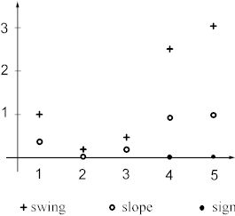
Figure 1. Example of results of method 1 ( maximal slope, swing and change of sign) for a single exemplar in a five dimensional input space.

We can compute the parameters for all the exemplars and average them to see if any patterns emerge. For example, higher value of swing for several coordinates may indicate that the inputs represented by these coordinates are more important in class separation than other inputs. If for most of the exemplars the slopes are steep and there are multiple boundaries along multiple directions, then the network may be overtrained and may not be able to generalize well.

The exemplars , which have the highest values of slopes and swings as well as point identified by input data analysis , e.g. centroids, ouliers etc. are good starting points for analysis by means of method 2 .

Method 2

In this method we look at 1-D and 2-D plots of the network functions. We select a point in the input space and one or two coordinates and plot the output of the network as a function of the selected coordinates. The tabulations make sense only for well selected points and coordinates. The choice can be best made using the input data analysis and the results of the method 1. The information provided by the tabulations is very useful in determining the shape of the function near class boundaries. Smooth and gradual transitions between flat plateaus are characteristic of well trained and well generalizing functions , see Figure 2(a).

Figure 2(a). A typical 1-D plot for a well generalizing network.

"Hesitant " transitions from uneven plateaus signify incompletely trained networks, see Figure 2(b).

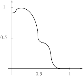
Figure 2(b). A typical 1-D plot for an incompletely trained network

Very sharp, multiple transitions signify an overtrained network with poor generalization, see Figure 2(c).

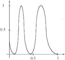Figure 2(c). A typical 1-D plot for an overtrained and poorly generalizing network

In concluding about the network character from the 1-D plots, one needs to keep in mind that they cover only a very small part of the total volume of the feasible input region.

Thus, we need to choose very carefully, which parts of the region need to be plotted and try to confirm our conclusions by means of other methods.

Method 3

In order to get a more complete picture of function in a vicinity of a selected input point we use a Monte Carlo test of class membership. In this test we sample the function around a given point and produce class membership of the sample points. This method produces information on a distance of the point to the nearest class boundary, and on the shape of the fragment of the boundary closest to it. By using dense sampling we can obtain detailed information about the function near selected points (e.g. outliers etc.), or with coarser sampling applied to a large number of points we can draw conclusions about generalization properties of the entire network.

3.0 ALGEBRAIC TECHNIQUES

3.1. APPROACH

The third class of methods of neural network analysis is based on techniques of linear algebra. These methods provides us with characterization of the neural network in respect to class separation and generalization properties. Neural network is highly nonlinear and in order to be able to use linear techniques we have to limit our analysis to one layer of the network. In particular we will analyze a matrix W ₁of weights between input and hidden neurons and a covariance matrix S of the hidden layer activations .

The algebraic methods support the information obtained by sensitivity analysis regarding the generalization properties of the network . For example , if the sensitivity analysis indicates presence of very complex class boundary, such that most of the exemplars lie near it and that most of them are surrounded by only a small region of the same class, then we may have a case of overfitting as a result of excessive number of neurons in the hidden layer. We can verify it by computing effective rank of matrix W ₁ or of covariance matrix S. The following two methods accomplish that task.

3.2 METHODS

Method 1

The following equation shows computation performed by the hidden layer of the neural network:

Y ₁= f ( W ₁* X ₁ ), (2)

where X ₁ is the input matrix, which columns are n-dimensional exemplars, matrix Y ₁is the matrix of hidden layer outputs, which m- dimensional columns are activations produced by hidden layer for each of the exemplars, W ₁ is an m x n matrix of weights between the input and hidden layer . Most of the networks used in ATR has smaller hidden layer than the input layer i.e. m < n. If W ₁ is rank deficient i.e. rank (W ₁ ) < m , then the outputs produced by the hidden layer will be linearly dependent. Thus some of the neurons are redundant.

We will determine the rank of W ₁by means of its singular value decomposition, shown below:

W ₁ = U ? V, (3)

where U and V are orthogonal and ? is an m x n diagonal matrix with m singular values on the diagonal sorted from the largest to the smallest. The number of significant singular values will determine the effective rank of the matrix.

We need to determine how many of the singular values are significant . In other words we need to set a threshold value, below which the singular values will be considered insignificant. If we keep k singular values and set to zero the remaining m-k values, than the right-hand side of equation 3 will provide the best, according to Frobenius norm, approximation of W ₁ of rank k. This leads us to the method of selecting the threshold value. We need to compute Frobenius norm of increment matrix ? W ₁ . This increment reflects the minimal resolution in weights computations caused by limited accuracy of the arithmetic and by the rate of weight update used in the training algorithm. Figure 3 shows an example of singular values and the threshold.

Figure 3. Sorted singular values and the threshold for network with five hidden neurons and effective rank of 3.

Method 2

This method provides alternative method of determining if there are redundancies in the hidden layer. We compute a covariance matrix S of the activation of the hidden layer:

S = cov ( W ₁* X ₁ ), (4)

where notation is as in equation (1). The matrix S is square and symmetric by definition and therefore has real eigenvalues. We perform eigenvalue decomposition of matrix S:

S = Q E Q ^T , (5)

where Q is orthogonal and E is a diagonal matrix of real eigenvalues. We use the absolute values of the eigenvalues to determine the number of significant eigenvalues and thus the rank of matrix S. Using reasoning very similar to that of method 1 we determine if there is redundancy in the hidden layer. This method supports the results obtained using method 1. If the rank obtained by this method is smaller than that of method 1, then it indicates that there are linear dependencies in the input data.

4.0 RULE EXTRACTION

4.1 APPROACH

This class of methods for analysis of neural netoworks is based on extraction of "if-then" rules from trained neural networks. We accomplish this by means of a method which determines the outcome of an existing rule linked with two rule extraction algorithms which provide successful ways of building rules from training exemplars.

All of our rules will be based on network behavior over rectangular regions. Throughout this paper, we assume that all input coordinates lie in the unit interval. By a rectangular region R, we mean a set of the form:

R = {x: x_i Î [ a _i, b _i], 0 < a _i < b _i < 1, i=1..n}.

Rectangular regions serve as input to the network at the input layer. If we let such sets propagate through the several layers of the network, we will refer to N(R) as their output in the final layer.

For a given output neuron, we are interested in assuring that the output belongs in a given class, e.g. high or low output. Hence, we ultimately wish to construct regions R such that

N(R) Í [0,0.5) or N(R) Í (0.5,1].

Therefore, an "if-then" rule for a multiple layer network is simply a statement of the form:

"if x Î R, then N(x) yields high output (i.e. in (0.5, 1])"

"If x Î (R₁ È R₂), then N(x) yields low output (i.e. in [0,0.5))".

The problem, of course, is that we can easily specify what output behavior we wish for our network, but we cannot so easily determine those sets R which yield that behavior.

So, how are we to go about constructing suitable input regions R?

One natural approach is to begin with the known behavior of our trained network. In other words, we can look to the training set of exemplars, each of whose output behavior is known. This collection of vectors and their outputs can be viewed as the set of seeds for "growing" input regions R.

Furthermore, we wish to build our input regions with maximum volume, so that the resulting rules will generate a compact approximation to the underlying implicit rule base being employed by the neural network.

By way of illustration, suppose we have a neural network with one output neuron and two input neurons which divides all inputs into one of two classes separated by some curve. See Figure 4.

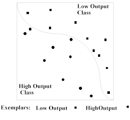
Figure 4. 2-D input space with two classes separated by a single boundary.

The ideal rule set for this network would specify the precise boundaries of each output region, particularly the functional definition of the curve that partitions the output space. The price of such precision, however, can be an unmanageable collection of rules which amount to a recitation of the coordinates of "all" of the points on the surface that separates the output classes. That is, if we demand to know the precise nature of the two output regions, we may end up with an impractical point by point representation of their boundary. Instead, our methods generate large rectangular regions whose union approximates the shape of these output regions. We opt for a small number of large rules rather than an exhaustive list of microscopic rules. See Figure 5.

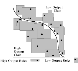Figure 5. 2-D input space withtwo classes separated by a single boundary and several rule regions in each class.

The techniques outlined in this chapter are applicable to arbitrary multiple layer neural networks. However, for discussion purposes, we will concentrate on trained neural networks having one hidden layer and one output neuron. The corresponding weight and bias matrices joining the input layer to hidden layer are denoted by W₁, b₁; while the weight and bias matrices joining the hidden and output layers will be denoted by W₂, b₂. We assume the activation function f(x) to be monotonic. For input vector x, the corresponding network y is given by:

y = N(x) = f(b₂ + S W₂ f(b₁ + S W₁x)).

In effect, the network acts as a map from the n-dimensional cube into the unit interval.

4.2 METHODS

The following theorem is instrumental in establishing that in any multiple layer network, N(R) is a single interval.

Theorem 1

Consider the connection between two consecutive layers of an arbitrary multiple layer neural network. Suppose the first layer has n neurons, connected by weight and bias matrices W and b to a given single neuron in the second layer. Let the first layer provide input to the second layer in the form of the region R = {x: x_i Î [ a _i, b _i], 0 < a _i < b _i < 1, i=1..n}.

Define c_i = a _i if W_i > 0, else b _i, i = 1..n, and d_i = b _i if W_i > 0, else a _i, i = 1..n.

Then, as we propagate R forward through the network, the corresponding output of the neuron in the second layer is the interval

[f(b + Wc), f( b + Wd)].

The proof of the theorem is relatively simple, and we will omit it for the sake of brevity of presentation.

By repeatedly applying the "forward propagation" approach of Theorem 1 to a multiple layer network, it is routine to see that the network output N(R) resulting from a closed rectangular input region R is a single, closed interval. The following example illustrates the process.

Demonstration

Consider a simple three layer network having 3 input neurons, 2 hidden layer neurons, and 1 output neuron with the indicated weights and biases. See Figure 6.

Assume also that we employ a log-sigmoidal activation function

f(x) = 1/(1 + exp(-x)).

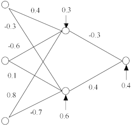
Figure 6. Example of a trained neural network.

Let the rectangular input region for this network be

R = [0, 0.3] x [0.1,0.8 ] x [0.6,1.0].

Theorem 1 tells us that when we forward propagate R from the input layer to the hidden layer, the output in the hidden layer will be

[0.574, 0.761] x [0.455, 0.565].

If we again use Theorem 1 to push this rectangle forward from the hidden layer to the single output neuron, we obtain

N(R) = [0.588, 0.699 ] as the final output of the network.

Growth Algorithms

We will now present two algorithms for creating regions R in [0,1]ⁿ such that N(R) Í (0.5,1] or

N(R) Í [0,0.5).

Our basic approach is to take an exemplar vector x for which N(x) Î (0.5,1], (say), and then "grow" a rectangular region R around x so that x Î R and

N(R) Í (0.5, 1].

We will examine two methods for growing regions around exemplars. They differ in the following respect: the first algorithm is based on growing a rule as a function of the local behavior of the derivative of the output with respect to individual input neurons. The second algorithm is based on growth in proportion to minimum and maximum boundaries of the rule.

Algorithm 1

Suppose we have an exemplar x whose output is in a known class. The simplest technique for "growing" a rectangular region around x, which also produces outputs in the same class, is to iteratively expand subintervals about each coordinate of x, symmetrically and uniformly.

We begin with a single exemplar, of type "high output", say, about which we iteratively build a rule by generating increasingly larger input intervals centered about the coordinates of the exemplar. This is done as follows: We select a growth increment, D , which is then repeatedly applied in both directions about each coordinate of the exemplar, as long as the corresponding output interval of the resulting region lies above the threshhold 0.5.

Rule Growth is controlled by three parameters:

1) a maximum rate, M, at which output interval endpoints are allowed to change as a function of input interval change,

2) a maximum width,W, of each input interval,

3) a minimum required distance or buffer, D, between the output interval and the 0.5 threshhold.

Here are the steps employed in one iteration of Algorithm 1:

1) For each coordinate, expand a symmetric interval about the exemplar coordinate value by the amount D in each direction.

2) Stop the growth on a given coordinate when one of the following conditions holds:

a) growth rate exceeds M, or

b) this coordinate’s interval width exceeds W, or

c) the distance between the ouput interval and the threshhold value of 0.5 is less than the D.

Steps 1 & 2 are repeated until there is no coordinate whose growth may continue.

Demonstration.

The idea is illustrated in Figure 7(a) - (c). Figure 7(a) shows a single high output exemplar.

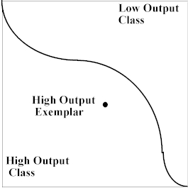
Figure 7(a). 2-D input space withtwo classes separated by a single boundary and a single exemplar.

Figure 7(b) shows the resulting rule R₁after one iteration of our algorithm. Here each coordinate has grown by an equal amount D , giving rise to a network output interval of, say,

N(R₁) = [0.55, 0.65].

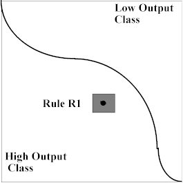
Figure 7(b). 2-D input space withtwo classes separated by a single boundary and an initial single rule.

In Figure 7(c), things get interesting. After many iterations of our algorithm, we begin to approach the curve that separates the classes. Because the boundary is closer horizontally than vertically, our rule R_khas slowed its horizontal growth, favoring continued vertical growth. This is typical of the growth behavior of intervals using this method, since we monitor the rate of growth as well as the distance to the output boundary. Furthermore, growth in the output interval is uneven as well (relative to the original exemplar output of 0.6), generating N(R_k) [0.51, 0.85]

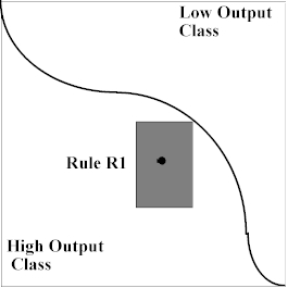
Figure 7(c). 2-D input space withtwo classes separated by a single boundary and a final single rule.

Discussion

The rate parameter M is an essential feature of this algorithm. It controls the maximum allowable value of the partial derivative of the output interval width as a function of each coordinate endpoint value. As the analysis in chapter 2 of this paper revealed, there can be vastly different sensitivity of the output to the different coordinates of the input. This growth algorithm takes that sensitivity into account in order that any individual interval does not grow too rapidly and thus jeopardize the overall rule growth.

Next, the width parameter W is a means of assuring that all intervals have nearly uniform width, thus preventing one or more intervals from dominating the overall growth of the rule to the exclusion of the growth of other coordinate intervals.

Finally, The threshhold buffer parameter D allows the user of the algorithm to control interval growth so that the output interval is maintained at any desired minimum distance from the 0.5 threshhold. As the use of the algorithm proceeds, one typically applies the algorithm with increasingly smaller values of the parameter D, after having observed the affect of the other two parameters, M and W.

Overall this rule is most useful when slow careful growth is required, such as when the derivative of the output of interval width with respect to each coordinate interval change is extremely sensitive, and especially when the exemplar is near the 0.5 threshhold, perhaps with respect to one or two key coordinates. This occurs especially in those cases when the boundary between high and low output exemplars is highly non-linear, so that subtle movements in individual coordinates move one violently from one domain set to another. Such careful growth procedures assure the creation of uniformly large coordinate intervals.

Algorithm 2

The next algorithm uses the minimum and maximum values of each exemplar coordinate to grow the rule. By minimum value, we mean the following: Suppose x = (x₁, x₂, ..., x_n) is a "high output" exemplar, then the minimum value, A_i , for coordinate i of x is given by

A_i = min (a _I) such that N({x₁, x₂, ..., x_i-1, [a _i,x_i], x_i+1, ..., x_n}) Ì (0.5, 1].

The maximum value, B_i, for coordinate i of x is given by

B_i = max (b _I) such that N({x₁, x₂, ...,

x_i-1,[x_i,b _i], x_i+1, ..., x_n }) Ì (0.5, 1].

For example, if N(x) Í (0.5,1], A_i is the smallest value of coordinate i of x such that if we propagate

R = {[x₁, x₁], [x₂, x₂], ..., [x_i-1, x_i-1],

[A_i, x_i], [x_i+1, x_i+1], ..., [x_n, x_n]} through the network we still obtain N(R) Í (0.5,1]. Note that R is thus a valid rule, but it only reflects growth of one end of one interval about one exemplar coordinate.

If we calculate all such minima and maxima, we obtain the region R_max/min = [A₁, B₁] x [A₂, B₂] x ... x [A_n, B_n]. This region represents the absolutely largest subset of [0,1]ⁿ for which N(R) is theoretically in the same class as x. It represents the largest rule one could hope to grow around x, one coordinate at a time.

It should be noted, however, that, in practice, N(R_max/min) is not even close to being in bounds. That is, usually N(R_max/min) has endpoints on opposite sides of 0.5. Thus, R_max/min does not represent a viable rule. However, R_max/min is useful in that represents a theoretical extremum toward which interval growth will be aimed in this algorithm.

Let us now consider how we may calculate R_max/minonce the overall growth has gotten under way. In general, as the algorithm proceeds and the growth has achieved a given viable rule, say,

I = [r₁, s₁] x [r₂, s₂] x ... x [r_n, s_n], we must re-evaluate the boundaries of R_{max/min .}This is done as follows: for each endpoint of I, we now hold all other subinterval endpoints of I fixed and then push our selected endpoint out to its minimum (for an r_j) or maximum (for an s_j) value while insisting that the resulting region correspond to a rule in the same class as the exemplar.

What remains, then is some explanation of how I is found. The details are given below.

This algorithm grows its intervals by taking steps in proportion to maximum available room for growth.

Suppose the present rule built thus far by this algorithm is

I = [r₁, s₁] x [r₂, s₂] x ... x [r_n, s_n].

We find R _max/min = [A₁, B₁] x [A₂, B₂] x ... x [A_n, B_n]. based on endpoint growth of rule I as described above.

A single step of Algorithm 2 involves the following:

The next rule generated by this algorithm is then:

J = [u₁, v₁] x [u₂, v₂] x ... x [u_n, v_n],

where, for each i=1..n, we have

r_i- u_i= k(r_i- A_i)

v_i - s_i= k(B_i - s_i),

where the constant k (0 < k < 1) is chosen so that the resulting rule J will still be valid, i.e. k is chosen so that N(J) is still in the same class as the exemplar x.

See Figure 8.

Figure 8. Growth of a 1-D interval according to Algorithm 2

In other words, we move from rule I to rule J by stretching each endpoint by an amount proportional to the distance between the current rule I and the min/max rule R _max/min.

This method terminates when the total growth gained by all intervals over the previous iteration is considered to be negligible.

Demonstration

For illustration, suppose we are given a neural network having two input neurons. See Figure 9.

As Algorithm 2 is applied, we begin with the exemplar state again as in Figure 7(a).

From the exemplar vector, we generate the extremum R _max/min depicted in Figure 9(a).

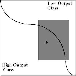
Figure 9(a). 2-D input space withtwo classes separated by a single boundary and the first maximal rule.

Suppose that, the proportionality constant is chosen to be k = 1/2. Thus, our first rule R₁ has half subintervals which are 1/2 of the lengths of the half intervals of R _max/min.We see the resulting rule in Figure 9(b),

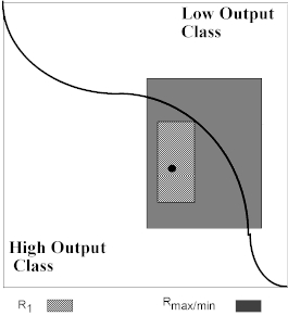
Figure 9(b). 2-D input space withtwo classes separated by a single boundary, the first maximal rule and the first ordinary rule.

Having created this first rule, we must recalculate R _max/min . This is done by holding each subinterval from rule R₁ fixed, then, one by one, moving each coordinate’s left and right endpoints outward until the output threshhold is reached. Figure 9(c) shows the newly calculated R _max/min.

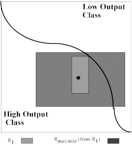
Figure 9(c). 2-D input space withtwo classes separated by a single boundary, the second maximal rule and the first ordinary rule.

At this point, we grow each coordinate interval , say, with the same proportionality constant k = 1/2, giving rise to the rule R₂ in Figure 9(d).

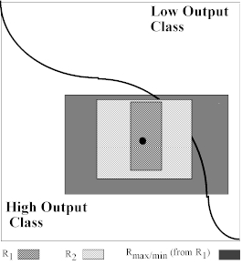
Figure 9(d). 2-D input space withtwo classes separated by a single boundary, the second maximal rule and the first and second ordinary rule.

Discussion

This rule takes careful note of the left and right boundaries of each coordinate. Its primary advantage is that it allows for balanced growth to occur in those cases where different coordinates have vastly different growth potential, independent of derivative behavior, but sensitive to growth extrema.

In a comparison of the two algorithms, one can see various comparative advantages. For example, if the derivatives are flat, then the first method is superior, whereas the second method is better for those sitations when the derivative is oscillatory but the boundaries are extreme.

Each of these techniques has been applied by the authors on a number of networks, yielding favorable and interesting results.

5.0 CONCLUSIONS

The paper addresses a problem of reliability of networks trained on small data sets. Users often hesitate to use these networks in real life situations relying only on their performance on a small number of test exemplars. It is therefore desirable to have some understanding of internal workings of a trained network. In particular, it is important to know how the network makes its classification decisions and what are its generalization properties. The methods presented in this paper aim at providing the necessary additional information about the network. They are to be used as a set in which any individual method provides only partial picture but as an ensemble they furnish significant insight . The methods come from three different approaches : sensitivity analysis, linear algebraic, and rule extraction. The methods have been captured in a toolbox programmed in Matlab and tested on a large number of real networks. They turned out to be very useful and helped significantly in evaluation of trained networks.

REFERENCES

[1] T.H Goh,., Francis Wong, "Semantic Extraction Using Neural Network Modeling and Sensitivity Analysis," ,"Proc. IEEE Intl. Joint Conference on Neural Networks, Singapore, 18-21 Nov. 1991.

[2] Sang-Hoon Oh, Youngjik Lee, "Sensitivity Analysis of Single Hidden-Layer Neural Networks," IEEE Transactions on Neural Networks, Vol. 6, NO. 4, 1005-1007, July 1995

[3] Y.H.Hu et al. "Structural Simplification of a Feed-forward, Multi-layer Perceptron Artificial Neural Network," ," Proc. IEEE Intl. Conference on Acoustics, Speech and Signal Processing 1991, pp. 1061-1064

[4] Quizhen Xue, Yu Hen Hu, Paul Milenkovic, " Analyses of the Hidden Units of the Multi-layer Perceptron and its Application in Acoustic-to-Articulatory Mapping," Proc. IEEE Intl. Conference on Acoustics, Speech and Signal Processing, 1990, pp. 869-872

[5] A.S. Weigend, D.E. Rumelhart, " The Effective Dimension of the Space of Hidden Units, "Proc. IEEE Intl. Joint Conference on Neural Networks, Singapore, 18-21 Nov. 1991, vol. 3 pp. 2069-2074

[6] Sebastian Thrun, "Extracting Symbolic Knowledge from Artificial Neural Networks," Advances in Neural Information Processing Systems, (NIPS) 1995.

[7] Peter Howes and Nigel Crook, "Rule Extraction from Neural Networks," Rules and Networks, Proceedings of the Rule Extraction From Trained Artificial Neural Networks Workshop, AISB, University of Sussex, 96. R. Andrews & J. Diederich (eds).